"”NONLINEAR SYSTEMS — COMPLETE NOTES””

ESSENTIAL MATRIX DERIVATIVE RULES

Matrix type	Form	Eigenvalues	Quick rule
Diagonal	`diag(a, d)`	$\lambda_1=a,\ \lambda_2=d$	Read off diagonal directly
Upper triangular	$\begin{bmatrix} a & b \\ 0 & d \end{bmatrix}$	$\lambda_1=a,\ \lambda_2=d$	Read off diagonal, ignore $b$
Lower triangular	$\begin{bmatrix} a & 0 \\ c & d \end{bmatrix}$	$\lambda_1=a,\ \lambda_2=d$	Read off diagonal, ignore $c$
Anti-diagonal	$\begin{bmatrix} 0 & b \\ c & 0 \end{bmatrix}$	$\lambda=\pm\sqrt{bc}$	$bc>0$: real saddle; $bc<0$: imaginary center
General $2\times2$	$\begin{bmatrix} a & b \\ c & d \end{bmatrix}$	$\lambda^2-\text{tr}\,\lambda+\det=0$	Use trace & determinant
Diagonal/Triangular $3\times3$	$\begin{bmatrix} a & * & * \\ 0 & d & * \\ 0 & 0 & f \end{bmatrix}$	$\lambda_1=a,\ \lambda_2=d,\ \lambda_3=f$	Read off diagonal directly
Anti-diagonal $3\times3$	$\begin{bmatrix} 0 & 0 & c \\ 0 & d & 0 \\ e & 0 & 0 \end{bmatrix}$	$\lambda_1=d,\ \lambda_{2,3}=\pm\sqrt{ce}$	Middle entry gives one $\lambda$; corner pair interact

INVERSE OF A $2\times2$ MATRIX

For

\[A=\begin{bmatrix} a & b \\ c & d \end{bmatrix},\qquad \det A = ad-bc,\]

the inverse exists iff $\det A\neq 0$, and is given by

\[A^{-1}=\frac{1}{ad-bc}\begin{bmatrix} d & -b \\ -c & a \end{bmatrix}.\]

Quick rule: swap the diagonal entries ($a\leftrightarrow d$), negate the off-diagonal entries ($b\to -b$, $c\to -c$), then divide by $\det A$.

Sanity check: $AA^{-1}=I$.

1.Derivative of a Transpose

Let $X = X(t)$.

\[\frac{d}{dt}(X^\top) = \left(\frac{dX}{dt}\right)^\top\]

2.Matrix Product Rule

\[\frac{d}{dt}(XY) = \dot X Y + X \dot Y\]

3.Quadratic Form

Let

\[V(x) = x^\top A x\]

Then

\[\nabla V(x) = (A + A^\top)x\]

If $A = A^\top$,

\[\nabla V(x) = 2Ax\]

4.Chain Rule (Lyapunov Use)

For

\[\dot x = f(x)\] \[\dot V(x) = \nabla V(x)^\top f(x)\]

1. Linear Systems

A linear time-invariant system:

System:

\[\dot{x} = A x\]

Solution:

\[x(t) = e^{At} x(0)\]

The stability of the system is determined by the eigenvalues $\lambda_i$ of $A$.

$\operatorname{Re}(\lambda_i) < 0$ for all $i$ $\Rightarrow$ asymptotically stable
$\operatorname{Re}(\lambda_i) > 0$ for some $i$ $\Rightarrow$ unstable
$\operatorname{Re}(\lambda_i) = 0$ for some $i$
- if the eigenvalues on the imaginary axis are simple $\Rightarrow$ Lyapunov stable
- otherwise $\Rightarrow$ unstable

Properties of linear systems:

Superposition principle holds
The equilibrium is typically unique: $x = 0$
No limit cycles exist
The global behavior is completely determined by the spectrum of $A$

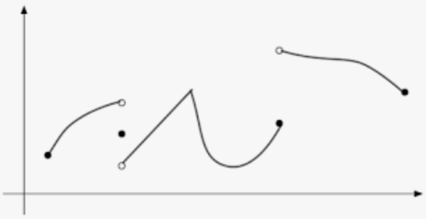
1.1 limit cycle

A limit cycle is an isolated periodic orbit of a nonlinear autonomous system

\[\dot{x} = f(x)\]

A trajectory $\gamma $ is a limit cycle if

it is periodic $\text{i.e. if there exists some } t_0 > 0 \text{ such that } x(t + t_0) = x(t) \text{ for all } t \in \mathbb{R}.$
there are no other periodic orbits arbitrarily close to it

Nearby trajectories may approach the orbit (stable), move away from it (unstable), or approach from one side only (semi-stable).

Limit cycles do not occur in linear systems.

Example

Consider the system in polar coordinates

\[\dot R = -R(R^2-1), \qquad \dot \theta = 1\]

Radial equilibria satisfy

\[\dot R = 0 \Rightarrow R = 0,\; R = 1\]

For $0<R<1$, $\dot R > 0 $ so the radius increases.
For $R>1$, $ \dot R < 0 $ so the radius decreases.

Thus trajectories move toward R=1 while $\theta $ keeps rotating.

The circle

\[R = 1\]

is therefore a stable limit cycle. you can have unstable one too if you like

2. Nonlinear Systems

General nonlinear autonomous system:

\[\dot{x} = f(x)\]

Equilibria satisfy:

\[f(x_e) = 0\]

Nonlinear systems may exhibit:

Multiple equilibria
Limit cycles
Bifurcations
Finite escape time
Complex attractors

Superposition does not hold:

\[f(x_1 + x_2) \neq f(x_1) + f(x_2)\]

Behavior depends on geometry of the vector field.

3. Normed Spaces

A norm satisfies:

$\Vert x\Vert \ge 0$, and $\Vert x\Vert =0 \iff x=0$
$\vert\alpha x\vert = \vert\alpha\vert\vert x\vert$
$\Vert x+y\Vert \le \Vert x\Vert +\Vert y\Vert $

Common norms in $\mathbb{R}^n$:

$\Vert x\Vert _2 = \sqrt{x^\top x}, \quad$ $\Vert x\Vert _1 = \sum |x_i|, \quad$ $\Vert x\Vert _\infty = \max_i |x_i|$

All norms are equivalent in finite dimensions.

4. Completeness

A sequence converges if:

\[\Vert x_n - x\Vert \to 0\]

(in strict definition: every ε>0, there exists an integer N such that for all n≥N the above <ε)

A sequence is Cauchy if:

\[\Vert x_n - x_m\Vert \to 0 \quad \text{as } n,m \to \infty\]

A space is complete if every Cauchy sequence converges in that space.

actually in $\mathbb{R}$ , every cauthy seq is converged.

A complete normed space is called a Banach space.

Completeness is required for fixed-point theorems.

5. Contraction Mapping

A mapping $P$ is a contraction if:

\[\Vert P(x)-P(y)\Vert \le L \Vert x-y\Vert , \quad 0 \le L < 1\]

Banach Fixed-Point Theorem

If $P$ is a contraction on a complete space:

A unique fixed point exists
x is cauthy and iteration converges to fixed point $x^*$

the P mapping could map the whole function to another function, so that the range contract (see homework)

6. Integral Form of ODE

Given:

\[\dot{x} = f(t,x), \quad x(t_0)=x_0\]

Integral form:

\[x(t)=x_0+\int_{t_0}^{t} f(s,x(s))\,ds\]

Define operator:

\[(Px)(t)=x_0+\int_{t_0}^{t} f(s,x(s))\,ds\]

Solving the ODE is equivalent to solving:

\[Px = x\]

Thus the ODE becomes a fixed-point problem.

7. Lipschitz Continuity

Global Lipschitz:

\[\Vert f(x)-f(y)\Vert \le L \Vert x-y\Vert\]

Local Lipschitz guarantees local existence and uniqueness.(with p.w. continuity)

piecewise continuity looks like not continued

Global Lipschitz guarantees global existence (the condition for no finite escape time).

how to find: take the derivative of f(x)

you can actually take the derivative of the linear system, then the answer is the lipschitz constant
lipschitz continuity $\rightarrow $ continuity

8. Finite Escape Time

Example:

\[\dot{x} = 1 + x^2\]

Solution:

\[x(t)=\tan t\]

Blow-up occurs at:

\[t=\frac{\pi}{2}\]

Conclusion:

Local Lipschitz ⇒ local solution
Global growth control ⇒ global solution

linear system does not have a finite escape time because the derivatives always a constant, so it is globally lipschitz $\rightarrow$ no finite escape time

9. Grönwall Inequality

\[u(t) \le C + \int_{t_0}^{t} a(s) u(s)\,ds\]

Then

\[u(t) \le C \exp\!\left(\int_{t_0}^{t} a(s)\,ds\right)\]

Used for:

Continuous dependence on IC
Growth bounds

10. Continuous Dependence on IC (Initial Conditions)

Four questions for nonlinear system:

solution exist?
solution unique?
have finite escape time?
continuous on IC?

Consider

\[\dot{x} = f(t,x), \quad x(t_0)=x_0\]

Assume:

$f$ is continuous in $t$
$f$ is locally Lipschitz in $x$

Then solutions depend continuously on the initial condition.

More precisely:

For $\forall$ $T>t_0$ and $\forall$ $\varepsilon>0$, there $\exists$ $\delta>0$ such that

\[\Vert x_0 - y_0\Vert < \delta \Rightarrow \sup_{t \in [t_0,T]} \Vert x(t,x_0) - x(t,y_0)\Vert < \varepsilon\]

This means small perturbations in the initial condition produce small changes in the entire trajectory over finite time intervals.

"”STABILITY THEORY””

11. Equilibrium

\[f(x_e)=0\]

12. Compactness

Close + bounded = compact

Example: [0,1]

13. Lyapunov Stability

Stable if:

For $\forall$ $\varepsilon>0$, there $\exists$ $\delta>0$ such that

\[\Vert x(0)-x_e\Vert <\delta \Rightarrow \Vert x(t)-x_e\Vert <\varepsilon\]

(Note: $t$ means any time $t \ge 0$, not $t \to \infty$)

Asymptotically stable if, first satisfied SISL, additionally:

\[\exists \delta > 0 \text{ s.t. } \|x_0\| < \delta \Rightarrow \|x(t, x_0)\| \to 0 \text{ as } t \to \infty\]

14. Lyapunov Direct Method

A scalar function $V(x)$ ( Lyapunov function )satisfies:

$V(x)>0$ for $x\neq 0$
$V(0)=0$

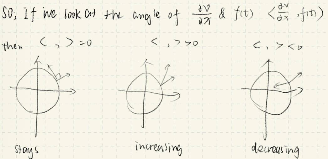
Derivative along trajectories:(basically $\dot x = f(x)$)

\[\dot{V}(x)=\nabla V(x)^\top f(x)\]

\[\dot{V}(x)\le 0\]

→ Stable.

\[\dot{V}(x)<0\]

→ Asymptotically stable.

intuition:

15. Global AS and LaSalle Theorem

If:

$V(x)>0$
$\dot{V}(x)\le 0$
$V(x)\to \infty$
as $x \to \infty$ (radially unbounded)

Then we say it is globally AS (remember the picture Prof draw in class)

LaSalle Thm preset

SISL
let $\mathcal{S}’= {x\in D \mid \dot V(x)=0 } $, if the only solution of the system dynamics within S is x(t)=$x_e$ = 0

then $x_e$ is AS

S is invariance set, in set S the $\dot{V} =0$, the other region in D is $\dot{V} <0$

this basically says the point will fall downward and fix only to the origin

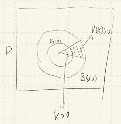
16. Instability Theorem (Chetaev)

If:

$V(0)=0$
$V(x)>0$
$\dot{V}(x)>0$ in a wedged region

or say:

in some point in the $B_\delta(X_e) $ $V(x)>0$,

and $\exists \varepsilon$ s.t. all $\dot{V}(x)$ >0 in this { $B_\epsilon(X_e)$ $\vert$ $V(x)>0$ }

Then equilibrium is unstable.

alt text

17. Lyapunov Equation

For the linearized system $\dot{x} = A(x - x_e),$

consider the quadratic Lyapunov function

\[V(x) = (x - x_e)^{\top} P (x - x_e),\]

where $P = P^{\top} > 0$.

The matrix $P$ satisfies the Lyapunov equation

\[A^{\top} P + P A = -Q,\]

where $Q = Q^{\top} > 0$. You can just assign $I$

If such a positive definite $P$ exists, then the equilibrium $x_e$ is locally asymptotically stable.

because the Lyapunov Equation makes

\[\dot{V} (x)= (x - x_e)^{\top} Q (x - x_e)<0\]

18. Linearization

Linearization matrix:

\[A = \frac{\partial f}{\partial x}\Big|_{x_e}\]

Approximation:

\[\dot{x} \approx A(x-x_e)\]

Linearization Example (Equilibrium Not at Origin)

Consider the nonlinear system

\[\begin{cases} \dot x_1 = x_2 \\ \dot x_2 = -x_1 + 1 - (x_1 - 1)^3 \end{cases}\]

1. Equilibrium

Solve

\[x_2 = 0, \quad -x_1 + 1 - (x_1 - 1)^3 = 0\]

We obtain

\[x_e = (1,0).\]

2. Jacobian

Let

\[f_1 = x_2, \quad f_2 = -x_1 + 1 - (x_1 - 1)^3.\]

Then

\[A(x) = \begin{bmatrix} 0 & 1 \\ -1 - 3(x_1 - 1)^2 & 0 \end{bmatrix}.\]

Evaluate at $x_e = (1,0) $:

\[J(x) = \begin{bmatrix} 0 & 1 \\ -1 & 0 \end{bmatrix}.\]

3. Linearized System

Define shifted state $(x-x_e)$

\[\tilde x = \begin{bmatrix} x_1 - 1 \\ x_2 \end{bmatrix}.\]

Then the linear approximation is

\[\dot{\tilde x} = \begin{bmatrix} 0 & 1 \\ -1 & 0 \end{bmatrix} \tilde x.\]

19. Lyapunov Indirect Method

After linearization,

If eigenvalues of $J(x)$:

$\forall$ Re(λ)<0 → locally asymptotically stable
$\exists$ Re(λ)>0 → unstable
$\exists$ Re(λ)=0 → inconclusive (cannot say SISL) (if the linear system neither grows nor decays → higher-order nonlinear terms decide, so the test is inconclusive.)

Indirect method is local.

20. Region of Attraction (ROA)

Defined as:

\[\mathcal{R} = \{x_0 : \lim_{t\to\infty} x(t,x_0)=0\}\]

Exact ROA is difficult to compute.

Using quadratic Lyapunov function:

\[V(x)=x^\top P x\]

sublevel set:

\[x^\top P x \le c\]

provides an inner estimate of ROA.

first V(x)is a lyapunov function
find biggest c s.t. $\dot{V} <0$ (for nonlinear you first linearize it, and then finding open ball for x in the case of nonlinear one, then calculate c base on your open ball x?)

look at home work

yes, and then calculate c using the following inequation

Formular:

$\because \lambda_{min} X^TX \le X^TPX \le \lambda_{max}X^TX $ and $x^\top P x \le c$

$\therefore $ $\lambda_{\min} \Vert x_{max} \Vert^2 \le c \;\Rightarrow\; \Vert x_{max} \Vert \le \sqrt{\frac{c}{\lambda_{\min}}}$

and

$\lambda_{\max} \Vert x_{min} \Vert^2 \le c \;\Rightarrow\; \Vert x_{min} \Vert \le \sqrt{\frac{c}{\lambda_{\max}}}$

"”Time-Varying System””

21. Stability of Time-Varying System

1.Time-Varying Systems

System: $\dot{x} = f(t,x)$

Equilibrium point: $\dot{x}\big|_{x_e} = 0 \;\Longleftrightarrow\; f(t,x_e)=0, \quad \forall t \ge t_0$

Region of Attraction (ROA): may depend on time (t), and can shrink.

2.Stability Definitions (Time-Varying)

1.Stability (SISL):

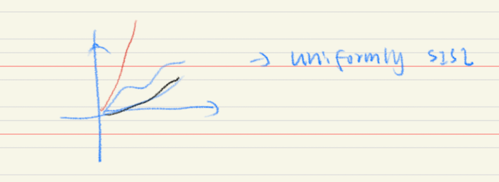
\[\forall \varepsilon > 0,\; \exists \delta(\varepsilon, t_0) > 0 \;\text{s.t.}\; \Vert x(t_0)\Vert < \delta \;\Rightarrow\; \Vert x(t)\Vert < \varepsilon,\; \forall t \ge t_0\]

2.Uniform stability:

\[\forall \varepsilon > 0,\; \exists \delta(\varepsilon) > 0 \;\text{s.t.}\; \Vert x(t_0)\Vert < \delta \;\Rightarrow\; \Vert x(t)\Vert < \varepsilon,\; \forall t \ge t_0\]

(note: $\delta$ does not depend on $t_0$)

Otherwise: unstable.

3.Asymptotic stability:

\[\exists \delta(t_0) > 0 \;\text{s.t.}\; \Vert x(t_0)\Vert < \delta \;\Rightarrow\; x(t) \to 0 \quad \text{as } t \to \infty\]

4.Uniform asymptotic stability:

\[\forall x_0\le c \\ \Vert x(t)\Vert \to 0 \quad \text{as } t \to \infty\]

independent of $t_0$

5.Global uniform asymptotic stability: $\Vert x(t)\Vert \to 0 \quad \text{as } t \to \infty$

Notes:

difference between uniform and normal one is the dependance of $t_0$

For normal (SISL) stability: $\forall \varepsilon>0,\;\exists \delta(\varepsilon,t_0)>0$ Here $\delta$ depends on $t_0$, so the system can behave differently if you start later. This is weaker.

For uniform stability: $\forall \varepsilon>0,\;\exists \delta(\varepsilon)>0$ Here $\delta$ is independent of $t_0$, so the same bound works for all starting times. This is stronger.

22. Class-$\mathcal{K}$ Functions

we introduce this to solve previous lyapunov conditions not working problems

1.class-$\mathcal{K}$

A function $\alpha:[0,a)\to[0,\infty)$ is class-$\mathcal{K}$ if:

Continuous
Strictly increasing
$\alpha(0)=0$

2.locally positive definite

A function $V : [0,\infty) \times \mathbb{R}^n \to \mathbb{R}$ is locally positive definite if

$V(t,0) = 0, \quad V(t,x) > 0 \;\; \forall x \ne 0,\; \forall t \ge 0$
there exists ( r > 0 ) and a class-$\mathcal{K}$ function $ \alpha : [0,r) \to [0,\infty) $

such that

\[V(t,x) \ge \alpha(\Vert x \Vert), \quad \forall t \ge 0,\; \forall x \in B_r(0)\]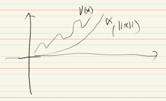

3.decrescent

A continuous function

\[V : [0,\infty) \times \mathbb{R}^n \to \mathbb{R}\]

is decrescent if there exists $ \delta > 0 $ and a class-$\mathcal{K}$ function

\[\gamma : [0,\infty) \to [0,\infty)\]

such that

\[V(t,x) \le \gamma(\Vert x \Vert), \quad \forall t \ge 0,\; \forall x \in B_\delta(0)\]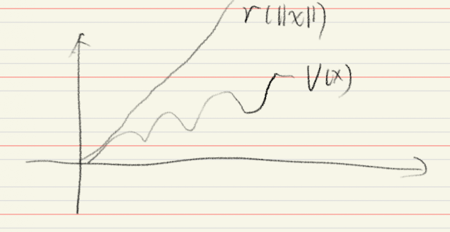

23. Lyapunov Conditions (Time-Varying)

(TFAE — The following are equivalent)

$V(t,x)$ is locally positive definite
$\exists\; W(x)$ locally positive definite such that

\[V(t,x) \ge W(x), \quad \forall t \ge 0,\; \forall x \in B_r(0)\]

define

\[\bar W(x) := \inf_{t \ge 0} V(t,x) \quad \text{is locally positive definite}\]

Consider the system

\[\dot{x} = f(t,x), \quad x(t_0)=x_0, \quad f(t,0)=0,\; \forall t \ge 0\]

Assume $f$ is locally Lipschitz in $x$ and piecewise continuous in $t$

1) Stability in the sense of Lyapunov (local)

If there exists a function (V(t,x)) such that:

local Positive definite: $\alpha_1(\|x\|) \le V(t,x)$
Non-increasing along trajectories: $\dot V = \frac{\partial V}{\partial t} + \frac{\partial V}{\partial x} f(t,x) \le 0$

then the equilibrium is locally Lyapunov stable.

2) Uniform Stability (Uniform SISL, local)

If in addition:

V is decrescent (upper bound independent of (t))

then the system is locally uniformly stable.

3) Asymptotic stability (non-uniform, local)

local Positive definite: $\alpha_1(\|x\|) \le V(t,x)$
$\dot{V}$ decreases along trajectories: $\dot V = \frac{\partial V}{\partial t} + \frac{\partial V}{\partial x} f(t,x) < 0$
Note: convergence may depend on initial time (t_0).

4) Uniform asymptotic stability (UAS, local)

To get uniformity (independent of initial time), require:

V decrescent

Then the system is locally uniformly asymptotically stable.

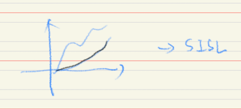
blue line is the trajectory.

24. Exponential Stability

1.ES

Equilibrium is exponentially stable if:

\[\Vert x(t)\Vert \le M e^{-\lambda t} \Vert x_0\Vert\]

for some $M>0$, $\lambda>0$.

2.Lyapunov condition(direct method):

If $c_1 \Vert x\Vert^2 \le V(x) \le c_2 \Vert x\Vert^2$ and $\dot{V}(x) \le -c_3 V(x)$, then exponentially stable.

3.Indirect Method (Linearization):

If $ A = \frac{\partial f}{\partial x}\Big|_{x=0} $ and all eigenvalues of $A$ satisfy $ \text{Re}(\lambda_i) < 0 $

then $x_e = 0$ is exponentially stable.

4.hierachy

\[\text{Exponential Stability} \Rightarrow \text{Asymptotic Stability} \Rightarrow \text{Stability}\]

Example: $\dot{x} = -x^3$ is asymptotically stable but NOT exponentially stable.

5.example of ES Example:

System $\dot{x} = -x^3$ is globally asymptotically stable (GAS), but convergence is slow (polynomial).
Add a small perturbation $\dot{x} = -x^3 + \varepsilon x$
Near $x=0$: $\dot{x} \approx \varepsilon x$ so the system becomes unstable.

Conclusion:

asymptotic stability can be destroyed by arbitrarily small perturbations
exponential stability is robust to small perturbations

Fix (via linearization):

design the system such that the linearization $A = \frac{\partial f}{\partial x}\Big|_{x=0}$ has eigenvalues satisfying $\text{Re}(\lambda_i) < 0$

So:

add a linear stabilizing term $\dot{x} = -x - x^3$
then near $x=0$, system behaves like $\dot{x} \approx -x$
so eigenvalue $\lambda = -1 < 0$ → ensures exponential stability and robustness

25. Linearization & Eigenvalue Test

Linearize system at equilibrium:

\[A = \frac{\partial f}{\partial x}\Big|_{x=0}\]

Stability determined by eigenvalues of $A$:

All $\text{Re}(\lambda) < 0$ → locally asymptotically stable (actually ES)
Any $\text{Re}(\lambda) > 0$ → unstable
$\text{Re}(\lambda) = 0$ → inconclusive (higher-order terms decide)

"”Control Method””

26. Control Lyapunov Function CLF

insight: How to control a system, makes it GAS

A lyapunov function $V(x)$ is a CLF if: $V(x) > 0,\quad V(0)=0$

and there exists control $u$ such that: $\inf_{u} \frac{\partial V}{\partial x} f(x,u) < 0,\quad \forall x \ne 0$

which is literally $\dot{V}(x)<0 $

Design: Choose $V(x)$ and design $u(x)$ to enforce $\dot{V}(x) < 0$.

27. Artstein Theorem (1983)

Consider: $\dot{x} = f(x,u)$

If:

$f$ is Lipschitz
there exists a CLF

then:

\[\exists \alpha(x) \in C^\infty\]

such that: $\dot{x} = f(x,\alpha(x))$

is GAS

only existence, not construction

28. Control Affine System

\[\dot{x} = f(x) + \sum_{i=1}^m g_i(x) u_i\]

\[\dot{x} = f(x) + g(x)u\]

and

\[y = h(x)\]

affine = linear + shift

29. Lie Derivative

\[L_f h(x) = \frac{\partial h}{\partial x} f(x)\]

For CLF: $\dot{V}(x) = L_f V(x) + \sum L_{g_i} V(x) u_i$

30. Key CLF Condition

\[\forall x \ne 0,\quad \inf_u \big[ L_f V(x) + L_g V(x) u \big] < 0\]

equivalent:

\[L_g V(x) = 0 \;\Rightarrow\; L_f V(x) < 0\]

if control cannot act, system must decay itself

31. Constructing Control

Goal: find $u = \alpha(x)$

\[u = \begin{cases} 0, & L_g V(x)=0 \\ -\dfrac{L_f V}{L_g V}, & L_g V(x)\ne 0 \end{cases}\]

min-norm controller

32. Small Control Property

A CLF satisfies:

\[\forall \epsilon>0,\ \exists \delta>0,\ \forall x\in B_\delta(0), x\ne0,\] \[\exists u,\ \Vert u\Vert < \epsilon\]

such that: $\dot V(x) < 0$

33. Sontag Control (GAS)

For: $\dot{x} = f(x) + g(x)u$

define: $u_s(x) = \begin{cases} \dfrac{-L_f V + \sqrt{(L_f V)^2 + (L_g V)^4}}{L_g V}, & L_g V \ne 0 \\ 0, & \text{otherwise} \end{cases}$

then: $\dot V(x) = -\sqrt{(L_f V)^2 + (L_g V)^4} < 0$

this input is contructed to ensures GAS

34. CLF vs Lyapunov

Lyapunov: $\dot{x} = f(x),\quad \dot V < 0$

CLF: $\dot{x} = f(x)+g(x)u,\quad \exists u:\dot V<0$

stability is not given, but achievable

35. Backstepping (idea)

stabilize system layer by layer

Introduce virtual control: $\dot{x} = f(x) + g(x)\xi,\quad \xi = u$

this is usually use when

actural u does not appear in the first equation, which means the first line is not directly controllable

such as

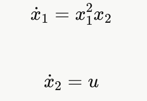alt text and

36. Backstepping Example

1.Backstepping Example (linear)

\[\begin{bmatrix} \dot{x}_1 \\ \dot{x}_2 \end{bmatrix} = \begin{bmatrix} 0 & 1 \\ - c_1 & -c_2 \end{bmatrix} \begin{bmatrix} x_1 \\ x_2 \end{bmatrix}\]

first write as this:

\[\dot{x}_1 = x_2, \qquad \dot{x}_2 = -c_1 x_1 - c_2 x_2\]

Choose virtual control:

\[x_2 = \alpha(x_1) = -c_1 x_1\]

2.Error Definition

\[z = x_2 - \alpha(x_1)\]

Then:

\[\dot{x}_1 = z - c_1 x_1\] \[\dot{z} = u + c_1(z - c_1 x_1)\]

3.Augmented Lyapunov

\[V_a(x,z) = \frac{1}{2}x_1^2 + \frac{1}{2}z^2\] \[\dot V_a = x_1\dot x_1 + z\dot z\]

Choose:

\[u = -x_1 - c_1(z - c_1 x_1) - c_2 z\] \[\Rightarrow \dot V_a < 0\]

4.Backstepping General Result

If:

$V(x)$ positive definite
radially unbounded

and

\[L_f V + L_g V \alpha(x) \le -W(x)\]

with $W(x)$ positive definite

then:

\[\text{closed-loop is GAS}\]

5.Integrator Backstepping Lemma

Augmented system:

\[\dot{x} = f(x) + g(x)\xi\] \[\dot{\xi} = u\]

Lyapunov:

\[V_a(x,\xi) = V(x) + \frac{1}{2}(\xi - \alpha(x))^2\]

6.Control Law (Backstepping)

\[u = - c(\xi - \alpha(x)) + \frac{\partial \alpha}{\partial x}(f(x)+g(x)\xi) - \frac{\partial V}{\partial x} g(x)\]

7.Weak Case (semi-definite)

If $W(x)$ is only positive semi-definite:

\[\dot V_a \le 0\]

then system converges to:

\[\mathcal{Z} = \{(x,\xi)\mid W(x)=0,\ \xi=\alpha(x)\}\]

not necessarily origin

37. Backstepping Revisit

Consider system:

\[\dot x = x \xi,\quad \dot \xi = u\]

Choose Lyapunov:

\[V(x) = \frac{1}{2}x^2\]

Let CLF:

\[V_a(x) = V(x) + \frac{1}{2}\xi^2\]

Then:

\[\dot V_a = x\dot x + \xi \dot \xi = \xi (x^2 + u)\]

Choose:

\[u = -x^2 - c\xi\]

Then:

\[\dot V_a = -c\xi^2 \le 0\]

Using LaSalle:

Invariant set:

\[S = \{(x,\xi)\mid \dot V_a = 0\} \Rightarrow \xi = 0\]

Then:

\[\dot \xi = u = -x^2\]

So:

\[\xi = 0 \Rightarrow x = 0\]

Only solution:

\[(x,\xi) = (0,0)\]

Therefore:

asymptotically stable

38. Strict Feedback System

Definition:

\[\dot x = f_0(x) + g_0(x)\xi_1\] \[\dot \xi_1 = f_1(x,\xi_1) + g_1(x,\xi_1)\xi_2\] \[\dot \xi_2 = f_2(x,\xi_1,\xi_2) + g_2(x,\xi_1,\xi_2)\xi_3\] \[\cdots\]

Assume:

\[f_i(0)=0\]

this is also backstepping

Each $\xi_i$ is a virtual control input

Goal:

make whole system GAS by ensuring $\dot V < 0$

39. Assumption A1

There exist:

\[\alpha(x),\; V(x)\]

such that:

\[\dot x = f_0(x) + g_0(x)\alpha(x)\]

is GAS (or SLS)

40. Backstepping Construction

Step 1:

\[\xi_1 = \alpha(x),\quad V_1(x)\]

Step 2:

\[\xi_2 = \alpha_1(x,\xi_1)\] \[V_2 = V_1(x) + \frac{1}{2}(\xi_1 - \alpha(x))^2\]

Step 3:

\[\xi_3 = \alpha_2(x,\xi_1,\xi_2)\] \[V_3 = V_2 + \frac{1}{2}(\xi_2 - \alpha_1)^2\]

General derivative:

\[\dot V_2 = \frac{\partial V_2}{\partial x}\dot x + \frac{\partial V_2}{\partial \xi_1}\dot \xi_1 + \frac{\partial V_2}{\partial \xi_2}\dot \xi_2\]

41. Sliding Mode Control (idea)

1.A simple system to discuss

System takes the form of:

\[\ddot y = -k y\]

Choose:

\[k = \pm 1\]

Goal:

\[y \to 0\]

Control:

$k$ switches between $\pm 1$

2.discussion of k=$\pm 1$

first, transform to State-space:

\[\dot x_1 = x_2\] \[\dot x_2 = -k x_1\]

For $k=1$: $\frac{dx_1}{dx_2} = -\frac{x_2}{x_1}$

Integrate: $x_1 dx_1 + x_2 dx_2 = 0$

\[\frac{x_1^2}{2} + \frac{x_2^2}{2} = C\]

circular trajectories (stable)

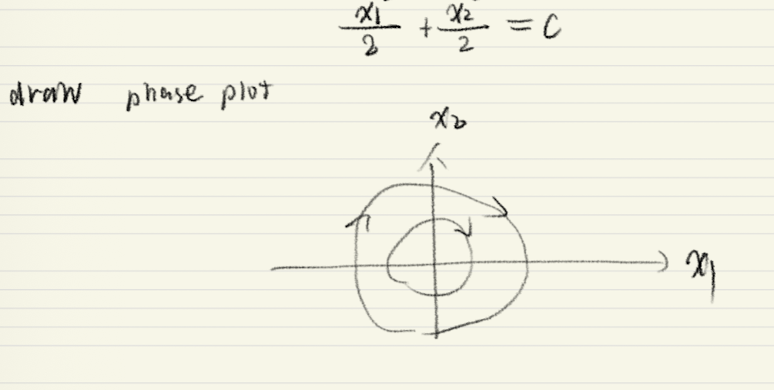
For $k=-1$: $\frac{x_1^2}{2} - \frac{x_2^2}{2} = C$

hyperbola (unstable)

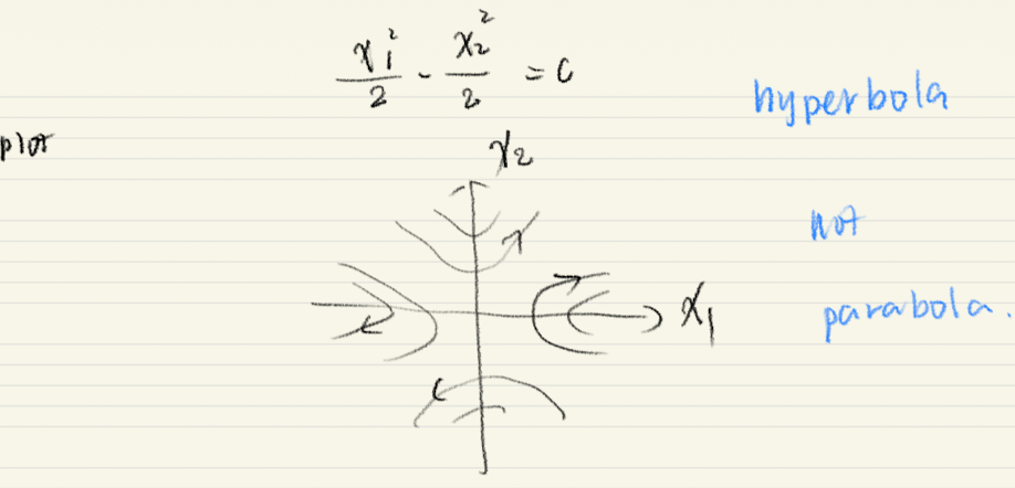
Conclusion:

switching needed

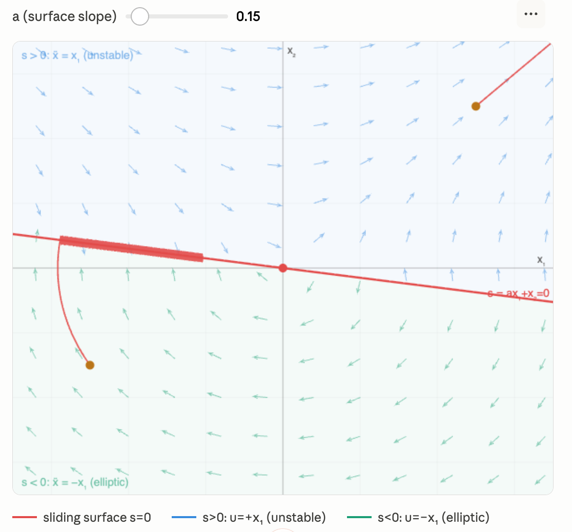
3.Sliding Surface

this surface is a surface because of the problem formation $\dot x_1 = x_2 $

Define:

\[s = a x_1 + x_2,\quad a>0\]

On surface $s=0$:

\[x_2 = -a x_1\]

Then:

\[\dot x_1 = -a x_1\]

So: $x_1 \to 0,\quad x_2 \to 0$

asymptotically stable on surface

General case for Sliding Mode Control

More General Example of Sliding Mode Control

2nd order system

\[\dot{x}_1 = x_2\] \[\dot{x}_2 = h(x) + g(x)u\]

if it is not this form, transform it first

$h$ and $g$ are unknown, but satisfied:

\[g(x) > g_0 > 0, \quad \forall x \in \mathbb{R}^2\]

Problem Statements

Design $u(x)$, s.t. $x = \begin{bmatrix} 0 \ 0 \end{bmatrix}$ is AS.

We do this by sliding mode control.

step 1: choosing sliding surface

\[s = a x_1 + x_2\] \[\dot s = a\dot x_1 + \dot x_2\] \[= a x_2 + h(x) + g(x)u\]

Assume:

\[\left|\frac{a x_2 + h(x)}{g(x)}\right| \le \delta(x),\quad \delta(x)>0 \tag{1}\]

step 2: Choose Lyapunov functon to ensure AS:

Pick Lyapunov function:

\[V(s) = \frac{1}{2}s^2\]

Then:

\[\dot{V} = s\dot{s} = s \cdot g(x) \cdot \frac{ax_2 + h(x)}{g(x)} + sg(x)u\] \[\leq g(x)|s| \cdot \delta(x) + sg(x)u\]

Choose:

\[u = -\beta(x)\,\text{sign}(x) \tag{2}\]

where:

\[\beta(x) \geq \beta_0 + \delta(x), \quad \beta_0 > 0\]

So:

\[\dot{V} \leq -g(x)\beta_0|s| \leq 0\]

Now we prove A.S. as long as the Assumption holds. Because we can choose a, so the assumption Equation (1) will hold.

Result

reaching mode: finite-time convergence to $s=0$
sliding surface: asymptotic convergence to origin

Conclusion

reaching phase: finite time
sliding phase: infinite time to $(0,0)$

Robustness

Control is robust to: $h(x),\; g(x)$

as long as assumption holds

42. Feedback Linearization

Motivation: General Problem

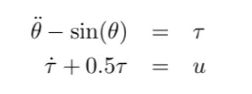
Consider a pendulum nonlinear system:

\[\dot{x_1} = x_2\] \[\dot{x}_2 = -a\sin x_1 - b x_2 + c u\]

Question: Can we design $u = u(x, v)$ to convert this into a linear system?

This is the idea behind feedback linearization.

2.def

If a system can be written as:

\[\dot{x} = A x + B r(x)[u - \alpha(x)]\]

Then we can choose:

\[u = \alpha(x) + r(x)^{-1} v\]

to achieve:

\[\dot{x} = A x + B v\]

which is linear.

3.Limitation Example

\[\dot{x}_1 = a \sin x_2\] \[\dot{x}_2 = -x_1^2 + u\]

We try to write it in the form:

\[\dot{x} = A x + B \gamma(x)\,[u - \alpha(x)]\]

However the nonlinearity $a \sin x_2$ appears in $\dot{x}_1$ and is not multiplied by the input $u$.

Example 2 (matrix form)

\[\dot{x} = \begin{bmatrix} \dot{x}_1 \\ \dot{x}_2 \end{bmatrix} = \begin{bmatrix} a \sin x_2 \\ - x_1^2 \end{bmatrix} + \begin{bmatrix} 0 \\ 1 \end{bmatrix} u\]

4.Solution: Coordinate Transformation

State transformation:

\[z_1 = x_1,\quad z_2 = a \sin x_2\]

Then:

\[\dot{z}_1 = z_2\] \[\dot{z}_2 = a \cos x_2 \cdot (-x_1^2 + u)\]

Input transformation - Choose:

\[u = x_1^2 + \frac{v}{a \cos x_2}\]

Resulting linear system:

\[\dot{z}_1 = z_2\] \[\dot{z}_2 = v\]

43. Formal Definition: Feedback Linearizable

A system

\[\dot{x} = f(x) + g(x) u\]

where f(x) denotes nonlinearity, g(x)is linearity.

is feedback linearizable if there exist:

A smooth control law: $u = \alpha(x) + \beta(x) v$
A coordinate transformation: $z = T(x)$

such that:

\[\dot{z} = A z + b v\]

for some constant matrices $A, b$.

Key questions:

When is a system feedback linearizable (checking $f, g$ only)?
What is the choice for $\alpha, \beta, T$?

Advantages and Defects:

Advantages: all linear control techniques can be used; easy recipe
Defects: requires knowing system dynamics $f, g$; may cancel stabilizing nonlinearity

44.Input-Output Linearization & Relative Degree

General SISO System

\[\dot{x} = f(x) + g(x) u\] \[y = h(x)\]

previously we do

\[u = \alpha(x) + r(x)^{-1} v\]

now if we make it simpler, instead of having all the state x linearized, we

We want output tracking: $y \to y_d$.

the Lie Derivatives

\[\dot{y} = L_f h(x)\] \[\ddot{y} = L_f^2 h(x) + L_g L_f h(x)\,u\]

Case 1: Relative Degree $r = 2$

If $L_g L_f h(x) \neq 0$, choose:

\[u = \frac{v - L_f^2 h(x)}{L_g L_f h(x)}\]

then:

\[\ddot{y} = v\]

Case 2: Relative Degree $r = 3$

If $L_g L_f h(x) = 0$ and $L_g L_f^2 h(x) \neq 0$, then:

\[y^{(3)} = L_f^3 h(x) + L_g L_f^2 h(x)\,u\]

Choose:

\[u = \frac{v - L_f^3 h(x)}{L_g L_f^2 h(x)}\]

then:

\[y^{(3)} = v\]

45. Zero Dynamics

\[\dot{x} = f(x) + g(x)u,\quad y = h(x)\]

Differentiate $y$ until $u$ appears (after $r$ times):

\[y^{(r)} = L_f^r h(x) + L_g L_f^{r-1} h(x)\,u\]

Choose $u$ to linearize the output channel ($\ddot y = v$):

\[u = \frac{v - L_f^r h(x)}{L_g L_f^{r-1} h(x)}\]

Let the output state vector be:

\[z = \begin{bmatrix} y \\ \dot y \\ \vdots \\ y^{(r-1)} \end{bmatrix} \in \mathbb{R}^r\]

Then:

\[\dot z = \begin{bmatrix} 0 & 1 & \cdots & 0 \\ \vdots & & \ddots & \vdots \\ 0 & 0 & \cdots & 1 \\ 0 & 0 & \cdots & 0 \end{bmatrix} z + \begin{bmatrix} 0 \\ \vdots \\ 0 \\ 1 \end{bmatrix} v\]

Choose linear control $v = -Kz$ so that $\dot z = (A - BK)z$ is stable, giving $z(t) \to 0$, thus $y(t) \to 0$.

Zero dynamics: the full state space is $n$-dimensional. The output makes $y = \dot y = \cdots = y^{(r-1)} = 0$ which solves $r$ dimensions. The remaining $n - r$ dimensions are not controlled by $v$ — their evolution on the manifold ${z = 0}$ is the zero dynamics.

To find zero dynamics: set $z = 0$ (i.e. $y = \dot y = \cdots = 0$), substitute $u^* = \frac{-L_f^r h(x)}{L_g L_f^{r-1} h(x)}$, and solve for the remaining $n-r$ states.

If zero dynamics are stable → full state converges → input-output linearization works
If zero dynamics are unstable → internal states blow up even as $y \to 0$ → system is non-minimum phase

46. Minimum Phase / Stability

\[\dot{x}_z = f_z(x_z)\] \[\text{zero dynamics stable} \;\Rightarrow\; \text{minimum phase}\] \[\text{zero dynamics unstable} \;\Rightarrow\; \text{non-minimum phase}\]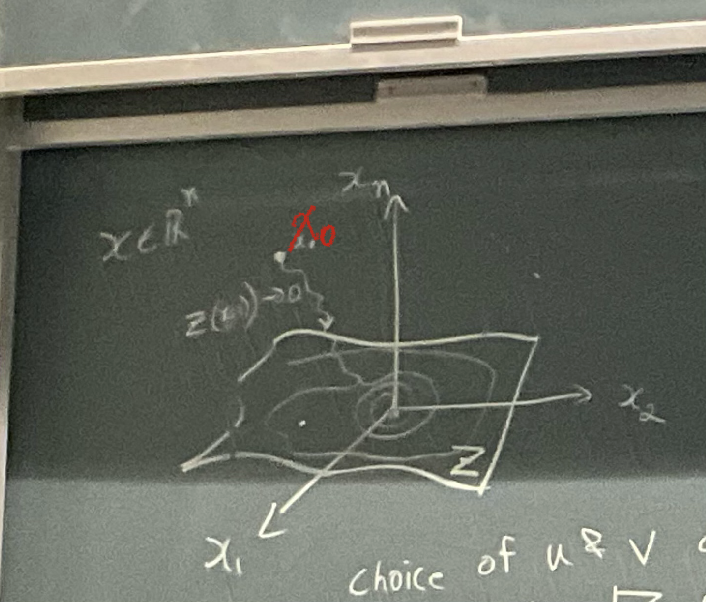

if we use z for vector [y, y’, y’’, …, y^(n-1)], this $\mathcal{Z}$ is the plane where $y = \dot y = \cdots = y^{(r-1)} = 0$ ,with dim of n-r

Example: Zero Dynamics + Pole-Zero

System:

\[\dot{x}_1 = x_2\] \[\dot{x}_2 = \alpha x_3 + u\] \[\dot{x}_3 = \beta x_3 - u\] \[y = x_1\]

Relative Degree

\[r = 2\]

Zero Dynamics

On manifold:

\[y = x_1 = 0\] \[\dot{y} = x_2 = 0\] \[\ddot{y} = 0\]

Solve for input:

\[\ddot{y} = \alpha x_3 + u = 0\] \[u^* = -\alpha x_3\]

Substitute into internal state:

\[\dot{x}_3 = \beta x_3 - u^*\] \[= \beta x_3 + \alpha x_3\] \[= (\alpha + \beta)x_3\]

Zero Dynamics

\[\dot{x}_3 = (\alpha + \beta)x_3\]

Stability

\[\alpha + \beta < 0 \Rightarrow \text{stable}\] \[\alpha + \beta > 0 \Rightarrow \text{unstable}\]

bonus Transfer Function

\[G(s) = \frac{s - (\alpha + \beta)}{s^2 (s - \beta)}\]

❓: how to get this

Relative Degree

\[r = 2\] \[r = \#\text{poles} - \#\text{zeros}\]

47. Conditions for Feedback Linearization

1.Introduction to Feedback Linearization

Consider a nonlinear system of the form:

\[\dot{x} = f(x) + g(x)u\]

The goal of feedback linearization is to transform this nonlinear system into an equivalent linear system through a change of coordinates and a feedback law.

Let the new coordinates be $z = \Phi(x)$ and the new input be $v$. We want to find a transformation such that the system dynamics in the new coordinates are linear:

\[\dot{z} = Az + Bv\]

If we can achieve this, we can use linear control techniques to control the system.

2.Differential Geometry Concepts

To understand feedback linearization, we need some concepts from differential geometry.

Manifold: A space that is locally Euclidean. For our purposes, the state space of the system can often be considered a manifold.
Vector Field: A function that assigns a tangent vector to each point on a manifold. In our system $\dot{x} = f(x)$, $f(x)$ is a vector field.
Lie Bracket: The Lie bracket of two vector fields $f$ and $g$, denoted as $[f, g]$, is another vector field defined as: $[f, g](x) = \frac{\partial g}{\partial x}f(x) - \frac{\partial f}{\partial x}g(x)$ The Lie bracket measures the non-commutativity of the flows of the vector fields. If $[f, g] = 0$, the vector fields are said to commute. (the vector fields are in a flat plane)
Adjoint: The adjoint operator is a way to represent repeated Lie brackets. $\text{ad}_f g(x) = [f, g](x)$ $\text{ad}_f^2 g(x) = [f, [f, g]](x)$ And in general: $\text{ad}_f^k g(x) = [f, \text{ad}_f^{k-1} g(x)]$
Distribution: A distribution $\Delta$ is a collection of vector subspaces of the tangent space at each point. For a set of vector fields ${g_1, \dots, g_m}$, the distribution is the span of these vector fields at each point $x$: $\Delta(x) = \text{span}\{g_1(x), \dots, g_m(x)\}$
Involutive Distribution: A distribution $\Delta$ is involutive if for any two vector fields $X, Y \in \Delta$, their Lie bracket $[X, Y]$ is also in $\Delta$.

3.Frobenius’ Theorem

A solution $h(x)$ to the PDE exists if the distribution

\[\Delta = \{ g, \operatorname{ad}_f g, \dots, \operatorname{ad}_f^{n-1} g \}\]

is involutive (Frobenius Theorem).

The core question When can we find a coordinate change $z = \Phi(x)$ that makes the system linear?
Lie bracket $[f,g](x) = \frac{\partial g}{\partial x}f(x) - \frac{\partial f}{\partial x}g(x)$

Measures how much two flow directions fail to commute — zero means the flows are flat relative to each other.

Distribution $\Delta$ $\Delta = \text{span}\{g,\, \text{ad}_f g,\, \ldots,\, \text{ad}_f^{n-1} g\}$

The set of all directions the system can be steered by input u— analogous to the controllability matrix.

Involutivity $\Delta$ is involutive if $X, Y \in \Delta \Rightarrow [X,Y] \in \Delta$.

$\Delta$ doesn’t “twist” — it defines a consistent flat submanifold everywhere in state space.

48. feedback linearizable THM

A system is feedback linearizable if and only if:

The matrix $\begin{bmatrix} g(x) & \text{ad}_f g(x) & \dots & \text{ad}_f^{n-1} g(x) \end{bmatrix}$ has rank $n$.
The distribution $D = \text{span}[g, \text{ad}_f g, \dots, \text{ad}_f^{n-2} g]$ is involutive.

If these conditions hold, we can find a function $h(x)$ such that:

\[\frac{\partial h}{\partial x} \begin{bmatrix} g(x) & \text{ad}_f g(x) & \dots & \text{ad}_f^{n-2} g(x) \end{bmatrix} = 0\]

The existence of such a solution $h(x)$ for the above Partial Differential Equation is guaranteed by Frobenius’ Theorem if the distribution $\Delta = {g, \dots, \text{ad}_f^{n-2} g}$ is involutive.

The PDE is: $\frac{\partial h}{\partial x} \cdot g(x) = 0, \quad \frac{\partial h}{\partial x} \cdot \text{ad}_f g(x) = 0, \quad \ldots, \quad \frac{\partial h}{\partial x} \cdot \text{ad}_f^{n-2} g(x) = 0$

Find a scalar $h(x)$ whose gradient is orthogonal to all vectors in $\Delta$ except the last one $\text{ad}_f^{n-1}g$. Once found, the full coordinate transformation is:

\[\Phi(x) = \begin{bmatrix} h(x) \\ L_f h(x) \\ \vdots \\ L_f^{n-1} h(x) \end{bmatrix}\]

Involutivity of $\Delta$ (Frobenius) guarantees this PDE has a consistent solution.

intuition: The two conditions together guarantee that a valid coordinate transformation $z = \Phi(x)$ exists.

Together: rank $n$ gives enough directions, involutivity makes them geometrically compatible. Both are necessary — rank without involutivity gives no valid $\Phi$, involutivity without rank means $\Phi$ exists but doesn’t cover the full state space.

49. Proof of Feedback Linearizability

To show that a system is feedback linearizable, we need to prove that it has a relative degree of $n$.

Lemma: A system has relative degree $n$ if and only if there exists a function $h(x)$ such that:

\[L_g L_f^k h(x) = 0, \quad \forall k = 0, \dots, n-2\] \[L_g L_f^{n-1} h(x) \neq 0\]

The existence of such a function $h(x)$ is guaranteed by Frobenius’ Theorem if the distribution $\Delta = \text{span}{g, \text{ad}_f g, \dots, \text{ad}_f^{n-2} g}$ is involutive.

Proof by Contradiction: Assume that $L_g h(x) = 0$. Then from the conditions for relative degree, we have:

\[\frac{\partial h}{\partial x} [g(x), \text{ad}_f g(x), \dots, \text{ad}_f^{n-1} g(x)] = [0, 0, \dots, L_g L_f^{n-1} h(x)]\]

If the matrix $[g(x), \text{ad}_f g(x), \dots, \text{ad}_f^{n-1} g(x)]$ has full rank, and we need $\frac{\partial h}{\partial x} \neq 0$ for a valid transformation, then we cannot have all elements on the right be zero. This implies that $L_g L_f^{n-1} h(x)$ cannot be zero, which confirms that the relative degree is $n$.

50. Example of Feedback Linearization

Goal: find $z = \Phi(x)$ such that in $z$-coordinates, $\dot z = Az + Bv$ (linear).

Step 1: Check controllability

\[\Delta = \text{span}\{g,\, \text{ad}_f g,\, \ldots,\, \text{ad}_f^{n-1} g\}\]

Must have rank $n$ — otherwise some directions are unreachable.

Step 2: Check involutivity

$\Delta$ must be involutive: $X, Y \in \Delta \Rightarrow [X,Y] \in \Delta$.

This guarantees the PDE for $h(x)$ has a solution (Frobenius theorem).

Step 3: Solve for $h(x)$

Find scalar $h(x)$ such that: $L_g h = 0,\quad L_g L_f h = 0,\quad \ldots,\quad L_g L_f^{n-2} h = 0, \quad L_g L_f^{n-1} h \neq 0$

$h(x)$ is the first coordinate of $z$ — everything else follows from it.

Step 4: Build $\Phi(x)$

\[z = \Phi(x) = \begin{bmatrix} h(x) \\ L_f h(x) \\ \vdots \\ L_f^{n-1} h(x) \end{bmatrix}\]

Because $\dot z_i = z_{i+1}$ must hold, each coordinate is just the time derivative of the previous one.

Step 5: Design $u$

\[u = \frac{v - L_f^n h(x)}{L_g L_f^{n-1} h(x)}\]

This cancels all nonlinearities, giving $z^{(n)} = v$.

Step 6: Linear control

\[v = -Kz \implies \dot z = (A - BK)z\]

Choose $K$ for desired eigenvalues.

Consider the system:

\[\dot{x} = \begin{bmatrix} a\sin(x_2) \\ -x_1^2 \end{bmatrix} + \begin{bmatrix} 0 \\ 1 \end{bmatrix} u\]

Here, $f(x) = \begin{bmatrix} a\sin(x_2) \ -x_1^2 \end{bmatrix}$ and $g(x) = \begin{bmatrix} 0 \ 1 \end{bmatrix}$.

Step 1: First, we check if the system is feedback linearizable. We compute the Lie bracket $[f, g]$:

\[[f, g] = \frac{\partial g}{\partial x}f - \frac{\partial f}{\partial x}g = 0 - \begin{bmatrix} 0 & a\cos(x_2) \\ -2x_1 & 0 \end{bmatrix} \begin{bmatrix} 0 \\ 1 \end{bmatrix} = \begin{bmatrix} -a\cos(x_2) \\ 0 \end{bmatrix}\]

The controllability matrix is:

\[\begin{bmatrix} g & [f,g] \end{bmatrix} = \begin{bmatrix} 0 & -a\cos(x_2) \\ 1 & 0 \end{bmatrix}\]

This matrix has rank 2 for all $x$ where $a\cos(x_2) \neq 0$.

Step 2: The distribution $\Delta = \text{span}{g}$ is involutive because for any scalar functions $\alpha(x), \beta(x)$, the Lie bracket $[\alpha g, \beta g]$ is in $\Delta$.

Step 3: Now we need to find $h(x)$ such that $L_g h(x) = 0$.

\[L_g h(x) = \nabla h \cdot g = \frac{\partial h}{\partial x_1} (0) + \frac{\partial h}{\partial x_2} (1) = \frac{\partial h}{\partial x_2} = 0\]

This implies that $h(x)$ is a function of $x_1$ only. Let’s choose $h(x) = x_1$.

Now we check the second condition:

\[L_g L_f h(x) = L_g ( \nabla h \cdot f) = L_g (a \ sin(x_2)) = \nabla(a \ sin(x_2)) \cdot g = \begin{bmatrix} 0 & a\cos(x_2) \end{bmatrix} \begin{bmatrix} 0 \\ 1 \end{bmatrix} = a\cos(x_2)\]

Since $L_g L_f h(x) \neq 0$ (in general), the system has relative degree 2 and is feedback linearizable.

Step 4: Build $\Phi(x)$

\[z = \Phi(x) = \begin{bmatrix} h(x) \\ L_f h(x) \end{bmatrix} = \begin{bmatrix} x_1 \\ a\sin(x_2) \end{bmatrix}\]

Step 5: Design $u$

Compute $L_f^2 h(x)$:

\[L_f^2 h = L_f(a\sin(x_2)) = \nabla(a\sin(x_2)) \cdot f = \begin{bmatrix} 0 & a\cos(x_2) \end{bmatrix} \begin{bmatrix} a\sin(x_2) \\ -x_1^2 \end{bmatrix} = -a x_1^2 \cos(x_2)\]

So:

\[u = \frac{v - L_f^2 h}{L_g L_f h} = \frac{v + ax_1^2\cos(x_2)}{a\cos(x_2)}\]

Step 6: Linear control

In $z$-coordinates the system is $\ddot z_1 = v$. Choose:

\[v = -k_1 z_1 - k_2 z_2 = -k_1 x_1 - k_2 a\sin(x_2)\]

giving closed-loop characteristic polynomial $s^2 + k_2 s + k_1$. Choose $k_1, k_2 > 0$ for stability.

51. MIMO Systems FB Lin

For Multi-Input Multi-Output (MIMO) systems, we consider a square system with $m$ inputs and $m$ outputs.

Q: why should it must in m*m?

because this way we could solve the inverse of decouple matrix A. This makes it like the SISO I/O Lin.

\[\dot{x} = f(x) + \sum_{j=1}^{m} g_j(x) u_j = f(x) + G(x)u\] \[y_i = h_i(x), \quad i=1, \dots, m\]

where $G(x) = [g_1(x), \dots, g_m(x)]$.

1.Vector Relative Degree

A MIMO system has a vector relative degree ${r_1, \dots, r_m}$ if:

$L_{g_j} L_f^k h_i(x) = 0$ for all $j=1, \dots, m$, for all $k < r_i - 1$, and for all $x$ in a neighborhood of $x_0$.
The $m \times m$ decoupling matrix $A(x) = \begin{bmatrix} L_{g_1}L_f^{r_1-1}h_1(x) & \dots & L_{g_m}L_f^{r_1-1}h_1(x) \\ \vdots & \ddots & \vdots \\ L_{g_1}L_f^{r_m-1}h_m(x) & \dots & L_{g_m}L_f^{r_m-1}h_m(x) \end{bmatrix}$ is nonsingular at $x=x_0$.

basically is taking the derivative of output $h_i$ exactly $r_i$ times.

If these conditions are met, we can define an input-output linearizing feedback law. The $i$-th output derivative is:

\[y_i^{(r_i)} = L_f^{r_i} h_i(x) + \sum_{j=1}^{m} L_{g_j} L_f^{r_i-1} h_i(x) u_j\]

In matrix form:

\[\begin{bmatrix} y_1^{(r_1)} \\ \vdots \\ y_m^{(r_m)} \end{bmatrix} = \begin{bmatrix} L_f^{r_1}h_1(x) \\ \vdots \\ L_f^{r_m}h_m(x) \end{bmatrix} + A(x) \begin{bmatrix} u_1 \\ \vdots \\ u_m \end{bmatrix}\]

By choosing $u = A(x)^{-1}(-b(x)+v)$, where $b(x)$ is the vector of $L_f^{r_i}h_i(x)$ terms, we can achieve $y_i^{(r_i)} = v_i$.

the reason why we need decoupling matrix to be full rank:

because that would mean our u (input) can control all m states. if it is not full rank, then, some rows are uncontrollable, thus making system failed

52. Final: State \ input \ output

\[\dot x = f(x, u), \qquad y = h(x)\]

Goal of control theory: use $u$ to drive $x$ as desired, using available $y$.

Method	What it does
Feedback linearization	use input to cancels nonlinearities in $\dot x = f(x)+g(x)u$ exactly. Requires full state + accurate model.
Input-output linearization	Differentiates OUTPUT $y=h(x)$ until input $u$ appears, cancels nonlinearities in the $y$-to-$u$ channel. state that are not cover(Zero dynamics) may be unstable.
Backstepping	Recursively stabilizes each state using virtual inputs, designs real $u$ at the last step.
Sliding mode	using input u which relate to sliding surface to Forces state onto surface $s=0$, then slides to origin. Robust to model uncertainty.

Feedback lin. vs Input-output lin.: Both cancel nonlinearities, but feedback linearization linearizes the full state dynamics while input-output linearization only linearizes the output response — leaving internal dynamics potentially unstable.