Policy Gradient & Actor-Critic Explained

PPO, TRPO, SAC, those contemporary algorithms build the foundation of today’s RL research. We see them in RL fine-tuning in Large Language Model, humanoid robots sim2real training and AI player plays chess game.

In order to give researcher a thorough understanding about how these groups of RL algorithms work, we will start from the intuitive Policy Gradient and Actor Critic, which is easier to connect back to ML and DL knowledge in mind. Then we dive deeper to each algorithm, since they are all traced back to the Policy Gradient and Actor Critic idea.

1. Policy Gradient (PG)

In a sense, doing deep learning is doing optimization to certain groups of parameters, and it’s no exception for Deep Reinforcement Learning. We formulate the idea as

\[\begin{align} \theta^* = \arg\max_{\theta} J(\theta) \end{align}\]

where

\[\begin{align} J(\theta) &= \mathbb{E}_{\tau \sim p_\theta(\tau)}\sum_{t=1}^{H} r(s_t, a_t)\\ &= \frac{1}{N} \sum_i \sum_t r(s_t^{(i)}, a_t^{(i)})\\ &= \int p_\theta(\tau) r(\tau) d\tau \end{align}\]

notice that (3) is a Monte Carlo estimate and (4) is the exact integral. So there is a sum & mean for N samples in (3) whereas (4) does not. (4) is purely the integration of every deterministic trajectory t , the N is hidden in the integral

Q1: what is $p_\theta$ here, what does it mean to do the sum and integral?

$\tau = (s_1, a_1, s_2, a_2, \ldots , s_H , a_H)$ is a trajectory sample from the policy $\pi_\theta$
$p_\theta(\tau) = \rho(s_1) \prod_{t=1}^{H} \pi_\theta(a_t \mid s_t) P(s_{t+1} \mid s_t , a_t)$ denotes the probability distribution of each $\tau$. This calculation is very intuitive, starting from state $s_1$, sample from $\pi_\theta$ for every $s_i$, $a_i$, times the state transitioning distribution $P(s’ \mid s , a)$

So now we can take the gradient of it, which is literally Policy Gradient, for future Back Propagation in a neural network.

\[\begin{align} \nabla J(\theta) &= \int \nabla_\theta p_\theta(\tau) \, r(\tau) \, d\tau \\ &= \int p_\theta(\tau)\, \nabla_\theta \log p_\theta(\tau)\, r(\tau) \, d\tau \\ &= \mathbb{E}_{\tau \sim p_\theta(\tau)} \nabla_\theta \log p_\theta(\tau)\, r(\tau) \end{align}\]

Now all we have is simply sample the trajectory from $p_\theta$ so we can get the $\nabla J(\theta)$. Then we do a gradient ascend on $\theta$

Q2: how to calculate the log item?

expanding the $p_?$ as we mentioned previously, take the derivative of the log item, then the objective function should be finally like

\[\begin{align} \nabla_\theta J(\theta) = \mathbb{E}_{\tau\sim p_\theta(\tau)}[(\sum\nabla_\theta log\pi_\theta(a|s)(\sum r (s,a))] \end{align}\]

here every single item is trackable. log item is calculate by PyTorch Autograd, and the reward item is from the system dynamics, such as predefine rules or functions.

2. Actor Critic

The difference of vanilla Policy Gradient and Actor Critic is whether there is a additional value function approximator by parameter $\phi $

alt text

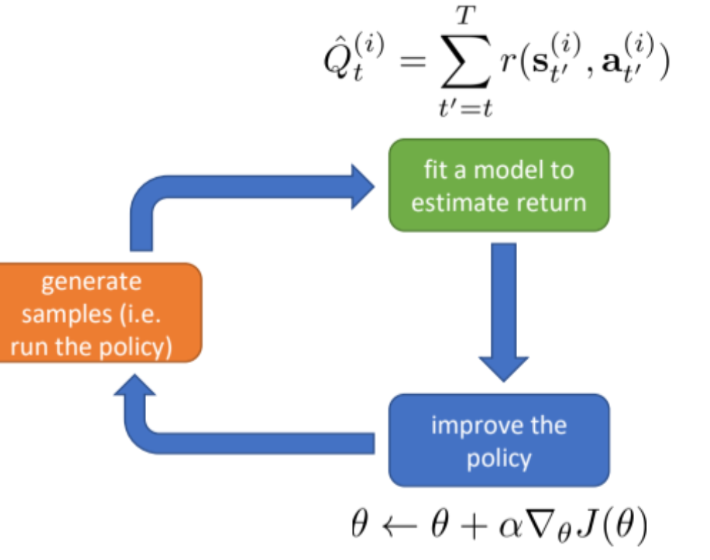
the vanilla PG

alt text

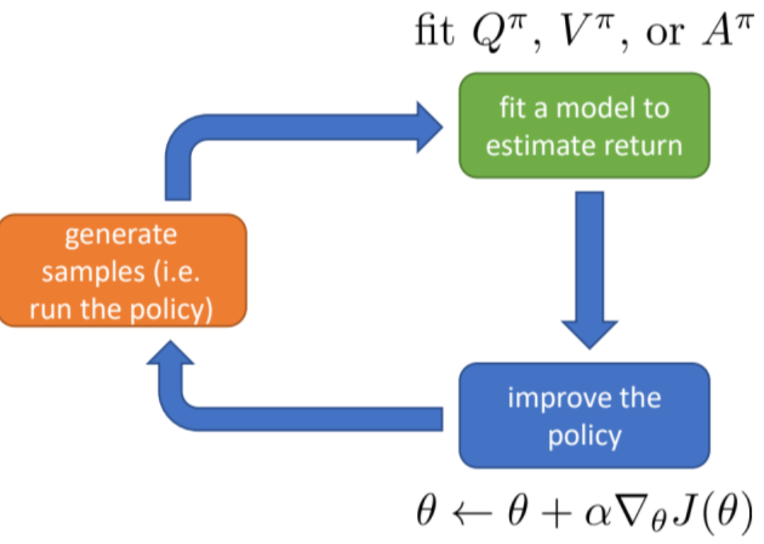
the Actor Critic

regarding the reward, which is the value function here, we have several steps to make it more precise, the final step is the introduction of actor critic

2.1. Advantage

\[\begin{align} A = Q(s_t,a_t)-V(s_t) \end{align}\]

this subtraction is to minus the average of Q (action value), which is a bias item for the value-function. think about when you in a chess game, when the starting position is already good, whatever moves you make, no matter how bad it is, could lead to a very high reward. That’s why we do need to subtract the bias term

\[\begin{align} A^\pi(s_t,a_t) &= Q(s_t,a_t)-V(s_t)\\ &= r(s_t,a_t)+V_\phi(s_{t+1})-V_\phi(s_t) \end{align}\]

2.2 Critic Network

now we fit the $A^\pi$ as the objective function of our critic network

\[\begin{align} \mathcal{L}(\phi)=\mathbb{E}[(\hat{V}^\pi_\phi(s_t^{(i)})-y_t^{(i)})^2] \end{align}\]

where $y_t^{(i)} = r(s_t,a_t)+\hat{V^\pi_\phi}(S_{t+1})$ . You can call it TD(temporal difference) target too

2.3 Actor Network

after fitting critic network in a single iteration, now we finally fit our actor model, namely our policy, here

the policy network optimization stays the same as Policy Gradient, which is

\[\begin{align} \nabla_\theta J(\theta) = \mathbb{E}_{\tau\sim p_\theta(\tau)}[(\sum\nabla_\theta log\pi_\theta(a|s)(\sum r (s,a))] \end{align}\]

So, the whole actor-critic algorithm should look like this

\begin{algorithm}
\caption{On-Policy Actor--Critic (TD)}
\begin{algorithmic}
\STATE Initialize $\theta, \phi$
\FOR{each iteration}
    \STATE Collect trajectories using $\pi_\theta$
    \FOR{each $(s_t,a_t,r_t,s_{t+1})$}
        \STATE $y_t = r_t + \gamma V_\phi(s_{t+1})$
        \STATE $\delta_t = y_t - V_\phi(s_t)$
        \STATE Update critic by minimizing $(V_\phi(s_t)-y_t)^2$
        \STATE $\theta \leftarrow \theta + \alpha \nabla_\theta \log \pi_\theta(a_t|s_t)\,\delta_t$
    \ENDFOR
\ENDFOR
\end{algorithmic}
\end{algorithm}